Subsetting Vectors

Krishnakanth Allika

2020-04-14 10:11

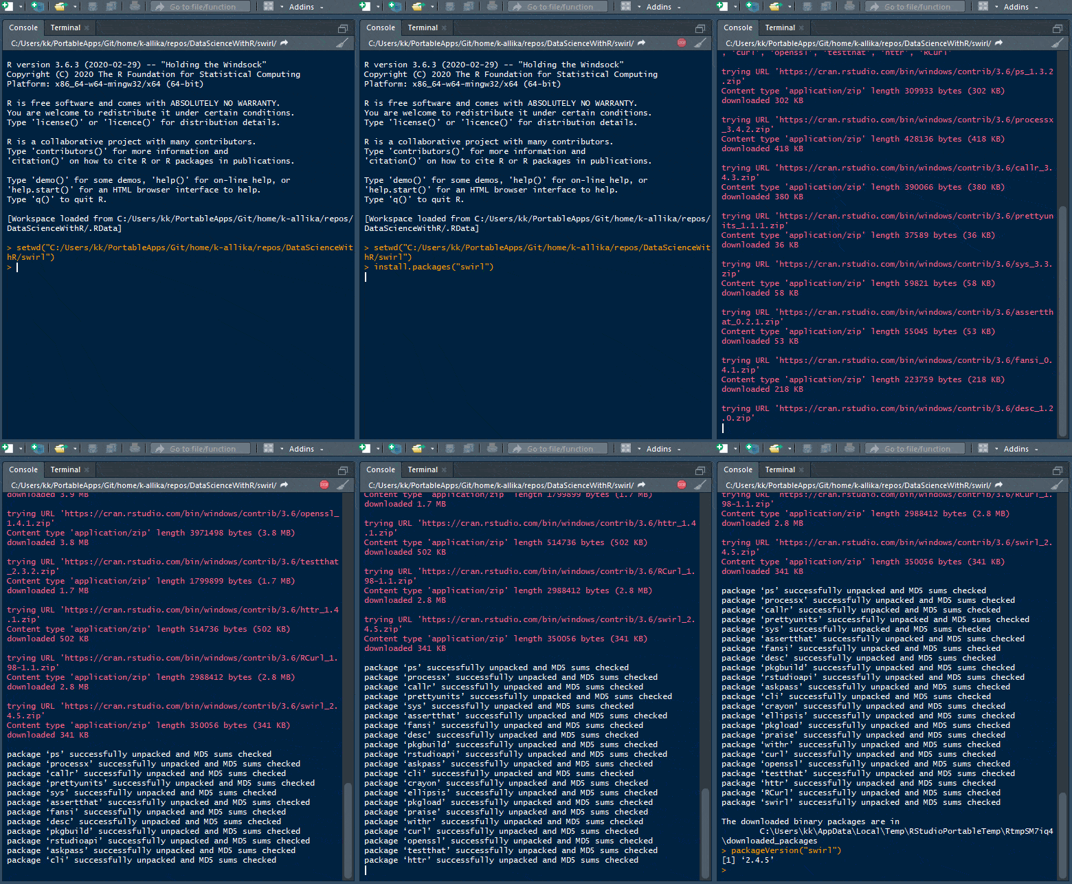
R version 3.6.3 (2020-02-29) -- "Holding the Windsock"
Copyright (C) 2020 The R Foundation for Statistical Computing
Platform: x86_64-w64-mingw32/x64 (64-bit)

R is free software and comes with ABSOLUTELY NO WARRANTY.
You are welcome to redistribute it under certain conditions.
Type 'license()' or 'licence()' for distribution details.

R is a collaborative project with many contributors.
Type 'contributors()' for more information and
'citation()' on how to cite R or R packages in publications.

Type 'demo()' for some demos, 'help()' for on-line help, or
'help.start()' for an HTML browser interface to help.
Type 'q()' to quit R.

[Workspace loaded from C:/Users/kk/PortableApps/Git/home/k-allika/repos/DataScienceWithR/.RData]

library("swirl")

| Hi! I see that you have some variables saved in your workspace. To keep things running
| smoothly, I recommend you clean up before starting swirl.

| Type ls() to see a list of the variables in your workspace. Then, type rm(list=ls()) to
| clear your workspace.

| Type swirl() when you are ready to begin.

ls()
[1] "my_char" "my_data" "my_div" "my_na" "my_name" "my_seq" "my_sqrt"
[8] "num_vect" "old.dir" "tf" "x" "y" "z"
rm(list=ls())
swirl()

| Welcome to swirl! Please sign in. If you've been here before, use the same name as you
| did then. If you are new, call yourself something unique.

What shall I call you? Krishnakanth Allika

| Please choose a course, or type 0 to exit swirl.

1: R Programming
2: Take me to the swirl course repository!

Selection: 1

| Please choose a lesson, or type 0 to return to course menu.

1: Basic Building Blocks 2: Workspace and Files 3: Sequences of Numbers
4: Vectors 5: Missing Values 6: Subsetting Vectors
7: Matrices and Data Frames 8: Logic 9: Functions
10: lapply and sapply 11: vapply and tapply 12: Looking at Data
13: Simulation 14: Dates and Times 15: Base Graphics

Selection: 6

| | 0%

| In this lesson, we'll see how to extract elements from a vector based on some
| conditions that we specify.

...

|== | 3%
| For example, we may only be interested in the first 20 elements of a vector, or only
| the elements that are not NA, or only those that are positive or correspond to a
| specific variable of interest. By the end of this lesson, you'll know how to handle
| each of these scenarios.

...

|==== | 5%
| I've created for you a vector called x that contains a random ordering of 20 numbers
| (from a standard normal distribution) and 20 NAs. Type x now to see what it looks like.

x
[1] -0.68754438 NA NA NA NA NA NA
[8] NA -0.01654302 1.03010195 -0.40799451 -0.55849418 NA -0.07687958
[15] -0.05351510 NA NA 1.16924926 1.60452324 -0.08284351 1.66735009
[22] NA NA 2.18942224 -0.14724334 NA NA -0.99999522
[29] NA NA -0.12665386 -0.61215464 -0.58919026 NA NA
[36] 1.12894965 -1.36770314 NA -1.33061090 NA

| You are amazing!

...

|======== | 10%
| For a simple example, try x[1:10] to view the first ten elements of x.

x[1:10]
[1] -0.68754438 NA NA NA NA NA NA
[8] NA -0.01654302 1.03010195

| You got it right!

|========== | 13%
| Index vectors come in four different flavors -- logical vectors, vectors of positive
| integers, vectors of negative integers, and vectors of character strings -- each of
| which we'll cover in this lesson.

...

|============ | 15%
| Let's start by indexing with logical vectors. One common scenario when working with
| real-world data is that we want to extract all elements of a vector that are not NA
| (i.e. missing data). Recall that is.na(x) yields a vector of logical values the same
| length as x, with TRUEs corresponding to NA values in x and FALSEs corresponding to
| non-NA values in x.

...

|============== | 18%
| What do you think x[is.na(x)] will give you?

1: A vector of length 0
2: A vector of all NAs
3: A vector of TRUEs and FALSEs
4: A vector with no NAs

Selection: 2

| That's the answer I was looking for.

|================ | 21%
| Prove it to yourself by typing x[is.na(x)].

x[is.na(x)]
[1] NA NA NA NA NA NA NA NA NA NA NA NA NA NA NA NA NA NA NA NA

| You got it!

|================== | 23%
| Recall that ! gives us the negation of a logical expression, so !is.na(x) can be read
| as 'is not NA'. Therefore, if we want to create a vector called y that contains all of
| the non-NA values from x, we can use y <- x[!is.na(x)]. Give it a try.

x[!is.na(x)]
[1] -0.68754438 -0.01654302 1.03010195 -0.40799451 -0.55849418 -0.07687958 -0.05351510
[8] 1.16924926 1.60452324 -0.08284351 1.66735009 2.18942224 -0.14724334 -0.99999522
[15] -0.12665386 -0.61215464 -0.58919026 1.12894965 -1.36770314 -1.33061090

| Nice try, but that's not exactly what I was hoping for. Try again. Or, type info() for
| more options.

| Type y <- x[!is.na(x)] to capture all non-missing values from x.

y<-x[!is.na(x)]

| You are doing so well!

|===================== | 26%
| Print y to the console.

y
[1] -0.68754438 -0.01654302 1.03010195 -0.40799451 -0.55849418 -0.07687958 -0.05351510
[8] 1.16924926 1.60452324 -0.08284351 1.66735009 2.18942224 -0.14724334 -0.99999522
[15] -0.12665386 -0.61215464 -0.58919026 1.12894965 -1.36770314 -1.33061090

| You are really on a roll!

|======================= | 28%
| Now that we've isolated the non-missing values of x and put them in y, we can subset y
| as we please.

...

|========================= | 31%
| Recall that the expression y > 0 will give us a vector of logical values the same
| length as y, with TRUEs corresponding to values of y that are greater than zero and
| FALSEs corresponding to values of y that are less than or equal to zero. What do you
| think y[y > 0] will give you?

1: A vector of all the negative elements of y
2: A vector of length 0
3: A vector of TRUEs and FALSEs
4: A vector of all NAs
5: A vector of all the positive elements of y

Selection: 5

| You are quite good my friend!

|=========================== | 33%
| Type y[y > 0] to see that we get all of the positive elements of y, which are also the
| positive elements of our original vector x.

y[y>0]
[1] 1.030102 1.169249 1.604523 1.667350 2.189422 1.128950

| All that practice is paying off!

|============================= | 36%
| You might wonder why we didn't just start with x[x > 0] to isolate the positive
| elements of x. Try that now to see why.

x[x>0]
[1] NA NA NA NA NA NA NA 1.030102 NA
[10] NA NA 1.169249 1.604523 1.667350 NA NA 2.189422 NA
[19] NA NA NA NA NA 1.128950 NA NA

| You are amazing!

|=============================== | 38%
| Since NA is not a value, but rather a placeholder for an unknown quantity, the
| expression NA > 0 evaluates to NA. Hence we get a bunch of NAs mixed in with our
| positive numbers when we do this.

...

|================================= | 41%
| Combining our knowledge of logical operators with our new knowledge of subsetting, we
| could do this -- x[!is.na(x) & x > 0]. Try it out.

x[!is.na(x)&x>0]
[1] 1.030102 1.169249 1.604523 1.667350 2.189422 1.128950

| You are really on a roll!

|=================================== | 44%
| In this case, we request only values of x that are both non-missing AND greater than
| zero.

...

|===================================== | 46%
| I've already shown you how to subset just the first ten values of x using x[1:10]. In
| this case, we're providing a vector of positive integers inside of the square brackets,
| which tells R to return only the elements of x numbered 1 through 10.

...

|======================================= | 49%
| Many programming languages use what's called 'zero-based indexing', which means that
| the first element of a vector is considered element 0. R uses 'one-based indexing',
| which (you guessed it!) means the first element of a vector is considered element 1.

...

|========================================= | 51%
| Can you figure out how we'd subset the 3rd, 5th, and 7th elements of x? Hint -- Use the
| c() function to specify the element numbers as a numeric vector.

x[c(3,5,7)]
[1] NA NA NA

| That's correct!

|=========================================== | 54%
| It's important that when using integer vectors to subset our vector x, we stick with
| the set of indexes {1, 2, ..., 40} since x only has 40 elements. What happens if we ask
| for the zeroth element of x (i.e. x[0])? Give it a try.

x[0]
numeric(0)

| Nice work!

|============================================= | 56%
| As you might expect, we get nothing useful. Unfortunately, R doesn't prevent us from
| doing this. What if we ask for the 3000th element of x? Try it out.

x[3000]
[1] NA

| Nice work!

|=============================================== | 59%
| Again, nothing useful, but R doesn't prevent us from asking for it. This should be a
| cautionary tale. You should always make sure that what you are asking for is within the
| bounds of the vector you're working with.

...

|================================================= | 62%
| What if we're interested in all elements of x EXCEPT the 2nd and 10th? It would be
| pretty tedious to construct a vector containing all numbers 1 through 40 EXCEPT 2 and
| 10.

...

|=================================================== | 64%
| Luckily, R accepts negative integer indexes. Whereas x[c(2, 10)] gives us ONLY the 2nd
| and 10th elements of x, x[c(-2, -10)] gives us all elements of x EXCEPT for the 2nd and
| 10 elements. Try x[c(-2, -10)] now to see this.

x[c(-2,-10)]
[1] -0.68754438 NA NA NA NA NA NA
[8] -0.01654302 -0.40799451 -0.55849418 NA -0.07687958 -0.05351510 NA
[15] NA 1.16924926 1.60452324 -0.08284351 1.66735009 NA NA
[22] 2.18942224 -0.14724334 NA NA -0.99999522 NA NA
[29] -0.12665386 -0.61215464 -0.58919026 NA NA 1.12894965 -1.36770314
[36] NA -1.33061090 NA

| That's a job well done!

|===================================================== | 67%
| A shorthand way of specifying multiple negative numbers is to put the negative sign out
| in front of the vector of positive numbers. Type x[-c(2, 10)] to get the exact same
| result.

x[-c(2,10)]
[1] -0.68754438 NA NA NA NA NA NA
[8] -0.01654302 -0.40799451 -0.55849418 NA -0.07687958 -0.05351510 NA
[15] NA 1.16924926 1.60452324 -0.08284351 1.66735009 NA NA
[22] 2.18942224 -0.14724334 NA NA -0.99999522 NA NA
[29] -0.12665386 -0.61215464 -0.58919026 NA NA 1.12894965 -1.36770314
[36] NA -1.33061090 NA

| Your dedication is inspiring!

|======================================================= | 69%
| So far, we've covered three types of index vectors -- logical, positive integer, and
| negative integer. The only remaining type requires us to introduce the concept of
| 'named' elements.

...

|========================================================= | 72%
| Create a numeric vector with three named elements using vect <- c(foo = 11, bar = 2,
| norf = NA).

vect<-c(foo=11,bar=2,norf=NA)

| You are amazing!

|=========================================================== | 74%
| When we print vect to the console, you'll see that each element has a name. Try it out.

vect
foo bar norf
11 2 NA

| That's a job well done!

|============================================================== | 77%
| We can also get the names of vect by passing vect as an argument to the names()
| function. Give that a try.

names(vect)
[1] "foo" "bar" "norf"

| Keep working like that and you'll get there!

|================================================================ | 79%
| Alternatively, we can create an unnamed vector vect2 with c(11, 2, NA). Do that now.

vect2<-c(11,2,NA)

| You are quite good my friend!

|================================================================== | 82%
| Then, we can add the names attribute to vect2 after the fact with names(vect2) <-
| c("foo", "bar", "norf"). Go ahead.

names(vect2)<-c("foo","bar","norf")

| Keep up the great work!

|==================================================================== | 85%
| Now, let's check that vect and vect2 are the same by passing them as arguments to the
| identical() function.

identical(vect,vect2)
[1] TRUE

| Keep up the great work!

|====================================================================== | 87%
| Indeed, vect and vect2 are identical named vectors.

...

|======================================================================== | 90%
| Now, back to the matter of subsetting a vector by named elements. Which of the
| following commands do you think would give us the second element of vect?

1: vect["2"]
2: vect["bar"]
3: vect[bar]

Selection: 2

| That's a job well done!

|========================================================================== | 92%
| Now, try it out.

vect["bar"]
bar
2

| You are doing so well!

|============================================================================ | 95%
| Likewise, we can specify a vector of names with vect[c("foo", "bar")]. Try it out.

vect[c("foo","bar",'norf')]
foo bar norf
11 2 NA

| You're close...I can feel it! Try it again. Or, type info() for more options.

| Use vect[c("foo", "bar")] to get only the elements of vect named "foo" and "bar".

vect[c("foo","bar")]
foo bar
11 2

| You are quite good my friend!

|============================================================================== | 97%
| Now you know all four methods of subsetting data from vectors. Different approaches are
| best in different scenarios and when in doubt, try it out!

...

|================================================================================| 100%
| Would you like to receive credit for completing this course on Coursera.org?

1: No
2: Yes

Selection: 2
What is your email address? xxxxxx@xxxxxxxxxxxx
What is your assignment token? xXxXxxXXxXxxXXXx
Grade submission succeeded!

| You got it right!

| You've reached the end of this lesson! Returning to the main menu...

| Please choose a course, or type 0 to exit swirl.

Last updated 2020-04-14 10:13:49.166837 IST

Missing Values

Krishnakanth Allika

2020-04-13 23:33

cache/posts/00405_Missing Values.html

swirl()

| Welcome to swirl! Please sign in. If you've been here before, use the same name as you
| did then. If you are new, call yourself something unique.

What shall I call you? Krishnakanth Allika

| Please choose a course, or type 0 to exit swirl.

1: R Programming
2: Take me to the swirl course repository!

Selection: 1

| Please choose a lesson, or type 0 to return to course menu.

Selection: 5

| | 0%

| Missing values play an important role in statistics and data analysis. Often, missing
| values must not be ignored, but rather they should be carefully studied to see if
| there's an underlying pattern or cause for their missingness.

...

|==== | 5%
| In R, NA is used to represent any value that is 'not available' or 'missing' (in the
| statistical sense). In this lesson, we'll explore missing values further.

...

|======== | 10%
| Any operation involving NA generally yields NA as the result. To illustrate, let's
| create a vector c(44, NA, 5, NA) and assign it to a variable x.

x<-c(44, NA, 5, NA)

| All that practice is paying off!

|============ | 15%
| Now, let's multiply x by 3.

x*3
[1] 132 NA 15 NA

| You are amazing!

|================ | 20%
| Notice that the elements of the resulting vector that correspond with the NA values in
| x are also NA.

...

|==================== | 25%
| To make things a little more interesting, lets create a vector containing 1000 draws
| from a standard normal distribution with y <- rnorm(1000).

y<-rnorm(1000)

| That's correct!

|======================== | 30%
| Next, let's create a vector containing 1000 NAs with z <- rep(NA, 1000).

z<-rep(NA,1000)

| You are doing so well!

|============================ | 35%
| Finally, let's select 100 elements at random from these 2000 values (combining y and z)
| such that we don't know how many NAs we'll wind up with or what positions they'll
| occupy in our final vector -- my_data <- sample(c(y, z), 100).

my_data<-sample(c(y,z),100)

| You nailed it! Good job!

|================================ | 40%
| Let's first ask the question of where our NAs are located in our data. The is.na()
| function tells us whether each element of a vector is NA. Call is.na() on my_data and
| assign the result to my_na.

my_na<-is.na(my_data)

| That's correct!

|==================================== | 45%
| Now, print my_na to see what you came up with.

my_na
[1] FALSE TRUE FALSE FALSE FALSE TRUE TRUE FALSE TRUE FALSE FALSE FALSE TRUE FALSE
[15] TRUE FALSE FALSE FALSE TRUE FALSE TRUE TRUE FALSE FALSE FALSE FALSE TRUE FALSE
[29] TRUE FALSE TRUE FALSE FALSE TRUE TRUE FALSE FALSE TRUE FALSE TRUE TRUE FALSE
[43] FALSE TRUE FALSE FALSE TRUE FALSE FALSE FALSE FALSE FALSE TRUE TRUE TRUE TRUE
[57] TRUE FALSE FALSE FALSE TRUE TRUE FALSE FALSE TRUE FALSE FALSE FALSE FALSE TRUE
[71] TRUE TRUE FALSE FALSE TRUE TRUE TRUE FALSE FALSE TRUE TRUE FALSE TRUE FALSE
[85] FALSE TRUE FALSE FALSE TRUE FALSE FALSE TRUE TRUE FALSE FALSE TRUE TRUE FALSE
[99] TRUE FALSE

| You are quite good my friend!

|======================================== | 50%
| Everywhere you see a TRUE, you know the corresponding element of my_data is NA.
| Likewise, everywhere you see a FALSE, you know the corresponding element of my_data is
| one of our random draws from the standard normal distribution.

...

|============================================ | 55%
| In our previous discussion of logical operators, we introduced the == operator as a
| method of testing for equality between two objects. So, you might think the expression
| my_data == NA yields the same results as is.na(). Give it a try.

my_data==NA
[1] NA NA NA NA NA NA NA NA NA NA NA NA NA NA NA NA NA NA NA NA NA NA NA NA NA NA NA NA
[29] NA NA NA NA NA NA NA NA NA NA NA NA NA NA NA NA NA NA NA NA NA NA NA NA NA NA NA NA
[57] NA NA NA NA NA NA NA NA NA NA NA NA NA NA NA NA NA NA NA NA NA NA NA NA NA NA NA NA
[85] NA NA NA NA NA NA NA NA NA NA NA NA NA NA NA NA

| All that hard work is paying off!

|================================================ | 60%
| The reason you got a vector of all NAs is that NA is not really a value, but just a
| placeholder for a quantity that is not available. Therefore the logical expression is
| incomplete and R has no choice but to return a vector of the same length as my_data
| that contains all NAs.

...

|==================================================== | 65%
| Don't worry if that's a little confusing. The key takeaway is to be cautious when using
| logical expressions anytime NAs might creep in, since a single NA value can derail the
| entire thing.

...

|======================================================== | 70%
| So, back to the task at hand. Now that we have a vector, my_na, that has a TRUE for
| every NA and FALSE for every numeric value, we can compute the total number of NAs in
| our data.

...

|============================================================ | 75%
| The trick is to recognize that underneath the surface, R represents TRUE as the number
| 1 and FALSE as the number 0. Therefore, if we take the sum of a bunch of TRUEs and
| FALSEs, we get the total number of TRUEs.

...

|================================================================ | 80%
| Let's give that a try here. Call the sum() function on my_na to count the total number
| of TRUEs in my_na, and thus the total number of NAs in my_data. Don't assign the result
| to a new variable.

sum(my_na)
[1] 43

| You're the best!

|==================================================================== | 85%
| Pretty cool, huh? Finally, let's take a look at the data to convince ourselves that
| everything 'adds up'. Print my_data to the console.

my_data
[1] -0.578578797 NA -0.112639140 0.836412196 -1.074043937 NA
[7] NA 1.303020726 NA 1.514220057 -1.533126560 -0.366673361
[13] NA -1.032058614 NA -1.631213149 0.379297612 -0.706613051
[19] NA -0.692352920 NA NA 0.535394170 -1.872906664
[25] -0.861449272 -1.321735747 NA -0.787816086 NA 0.801388943
[31] NA -1.487792282 0.470028145 NA NA 1.187583726
[37] -1.704604005 NA 0.596807280 NA NA -1.493099149
[43] 0.265671235 NA -0.985396879 -0.974373033 NA 1.377397659
[49] -0.637308342 -1.450105656 0.192263390 0.776355028 NA NA
[55] NA NA NA 1.567478781 -0.511602362 0.107048330
[61] NA NA -0.408394399 0.592123817 NA 0.305403550
[67] 3.201114883 0.806735141 0.698544788 NA NA NA
[73] -2.671330480 0.123440813 NA NA NA -1.236370155
[79] 0.936670598 NA NA 1.519229128 NA -1.366810674
[85] 0.211749069 NA 0.203741812 1.319234085 NA -0.432928319
[91] -0.006566875 NA NA 0.060568295 0.292428312 NA
[97] NA 0.717821949 NA 0.359249723

| You're the best!

|======================================================================== | 90%
| Now that we've got NAs down pat, let's look at a second type of missing value -- NaN,
| which stands for 'not a number'. To generate NaN, try dividing (using a forward slash)
| 0 by 0 now.

0/0
[1] NaN

| That's a job well done!

|============================================================================ | 95%
| Let's do one more, just for fun. In R, Inf stands for infinity. What happens if you
| subtract Inf from Inf?

Inf-Inf
[1] NaN

| You are really on a roll!

|================================================================================| 100%
| Would you like to receive credit for completing this course on Coursera.org?

1: Yes
2: No

Selection: 1
What is your email address? xxxxxx@xxxxxxxxxxxx
What is your assignment token? xXxXxxXXxXxxXXXx
Grade submission succeeded!

| You are doing so well!

| You've reached the end of this lesson! Returning to the main
| menu...

| Please choose a course, or type 0 to exit swirl.

Last updated 2020-04-13 23:32:50.765370 IST

Vectors

Krishnakanth Allika

2020-04-13 23:31

cache/posts/00404_Vectors.html

swirl()

| Welcome to swirl! Please sign in. If you've been here before, use the same name as you
| did then. If you are new, call yourself something unique.

What shall I call you? Krishnakanth Allika

| Please choose a course, or type 0 to exit swirl.

1: R Programming
2: Take me to the swirl course repository!

Selection: 1

| Please choose a lesson, or type 0 to return to course menu.

Selection: 4

| | 0%

| The simplest and most common data structure in R is the vector.

...

|== | 3%
| Vectors come in two different flavors: atomic vectors and lists. An atomic vector
| contains exactly one data type, whereas a list may contain multiple data types. We'll
| explore atomic vectors further before we get to lists.

...

|==== | 5%
| In previous lessons, we dealt entirely with numeric vectors, which are one type of
| atomic vector. Other types of atomic vectors include logical, character, integer, and
| complex. In this lesson, we'll take a closer look at logical and character vectors.

...

...

|======== | 11%
| First, create a numeric vector num_vect that contains the values 0.5, 55, -10, and 6.

num_vect<-c(0.5, 55, -10, 6)

| All that hard work is paying off!

|=========== | 13%
| Now, create a variable called tf that gets the result of num_vect < 1, which is read as
| 'num_vect is less than 1'.

tf<-num_vect<1

| You are really on a roll!

|============= | 16%
| What do you think tf will look like?

1: a vector of 4 logical values
2: a single logical value

Selection: 1

| Your dedication is inspiring!

|=============== | 18%
| Print the contents of tf now.

tf
[1] TRUE FALSE TRUE FALSE

| That's correct!

|================= | 21%
| The statement num_vect < 1 is a condition and tf tells us whether each corresponding
| element of our numeric vector num_vect satisfies this condition.

...

|=================== | 24%
| The first element of num_vect is 0.5, which is less than 1 and therefore the statement
| 0.5 < 1 is TRUE. The second element of num_vect is 55, which is greater than 1, so the
| statement 55 < 1 is FALSE. The same logic applies for the third and fourth elements.

...

|===================== | 26%
| Let's try another. Type num_vect >= 6 without assigning the result to a new variable.

num_vect>=6
[1] FALSE TRUE FALSE TRUE

| Great job!

|======================= | 29%
| This time, we are asking whether each individual element of num_vect is greater than OR
| equal to 6. Since only 55 and 6 are greater than or equal to 6, the second and fourth
| elements of the result are TRUE and the first and third elements are FALSE.

...

|========================= | 32%
| The < and >= symbols in these examples are called 'logical operators'. Other
| logical operators include >, <=, == for exact equality, and != for inequality.

...

|=========================== | 34%
| If we have two logical expressions, A and B, we can ask whether at least one is TRUE
| with A | B (logical 'or' a.k.a. 'union') or whether they are both TRUE with A & B
| (logical 'and' a.k.a. 'intersection'). Lastly, !A is the negation of A and is TRUE when
| A is FALSE and vice versa.

...

|============================= | 37%
| It's a good idea to spend some time playing around with various combinations of these
| logical operators until you get comfortable with their use. We'll do a few examples
| here to get you started.

...

|================================ | 39%
| Try your best to predict the result of each of the following statements. You can use
| pencil and paper to work them out if it's helpful. If you get stuck, just guess and
| you've got a 50% chance of getting the right answer!

...

|================================== | 42%
| (3 > 5) & (4 == 4)

1: FALSE
2: TRUE

Selection: 1

| That's correct!

|==================================== | 45%
| (TRUE == TRUE) | (TRUE == FALSE)

1: FALSE
2: TRUE

Selection: 2

| You are quite good my friend!

|====================================== | 47%
| ((111 >= 111) | !(TRUE)) & ((4 + 1) == 5)

1: FALSE
2: TRUE

Selection: 1

| Not exactly. Give it another go.

| This is a tricky one. Remember that the ! symbol negates whatever comes after it.
| There's also an 'order of operations' going on here. Conditions that are enclosed
| within parentheses should be evaluated first. Then, work your way outwards.

1: FALSE
2: TRUE

Selection: 2

| You nailed it! Good job!

|======================================== | 50%
| Don't worry if you found these to be tricky. They're supposed to be. Working with
| logical statements in R takes practice, but your efforts will be rewarded in future
| lessons (e.g. subsetting and control structures).

...

|========================================== | 53%
| Character vectors are also very common in R. Double quotes are used to distinguish
| character objects, as in the following example.

...

|============================================ | 55%
| Create a character vector that contains the following words: "My", "name", "is".
| Remember to enclose each word in its own set of double quotes, so that R knows they are
| character strings. Store the vector in a variable called my_char.

my_char<-c( "My", "name", "is")

| You're the best!

|============================================== | 58%
| Print the contents of my_char to see what it looks like.

my_char
[1] "My" "name" "is"

| Great job!

|================================================ | 61%
| Right now, my_char is a character vector of length 3. Let's say we want to join the
| elements of my_char together into one continuous character string (i.e. a character
| vector of length 1). We can do this using the paste() function.

...

|=================================================== | 63%
| Type paste(my_char, collapse = " ") now. Make sure there's a space between the double
| quotes in the collapse argument. You'll see why in a second.

paste(my_char,collapse = " ")
[1] "My name is"

| Great job!

|===================================================== | 66%
| The collapse argument to the paste() function tells R that when we join together the
| elements of the my_char character vector, we'd like to separate them with single
| spaces.

...

|======================================================= | 68%
| It seems that we're missing something.... Ah, yes! Your name!

...

|========================================================= | 71%
| To add (or 'concatenate') your name to the end of my_char, use the c() function like
| this: c(my_char, "your_name_here"). Place your name in double quotes where I've put
| "your_name_here". Try it now, storing the result in a new variable called my_name.

my_name<-c(my_char,"Krishnakanth Allika")

| You are doing so well!

|=========================================================== | 74%
| Take a look at the contents of my_name.

my_name
[1] "My" "name" "is"
[4] "Krishnakanth Allika"

| That's the answer I was looking for.

|============================================================= | 76%
| Now, use the paste() function once more to join the words in my_name together into a
| single character string. Don't forget to say collapse = " "!

paste(my_name,collapse = " ")
[1] "My name is Krishnakanth Allika"

| You got it!

|=============================================================== | 79%
| In this example, we used the paste() function to collapse the elements of a single
| character vector. paste() can also be used to join the elements of multiple character
| vectors.

...

|================================================================= | 82%
| In the simplest case, we can join two character vectors that are each of length 1 (i.e.
| join two words). Try paste("Hello", "world!", sep = " "), where the sep argument
| tells R that we want to separate the joined elements with a single space.

paste("Hello","world!",sep=" ")
[1] "Hello world!"

| Keep up the great work!

|=================================================================== | 84%
| For a slightly more complicated example, we can join two vectors, each of length 3. Use
| paste() to join the integer vector 1:3 with the character vector c("X", "Y", "Z"). This
| time, use sep = "" to leave no space between the joined elements.

paste(1:3,c("X", "Y", "Z"),sep="")
[1] "1X" "2Y" "3Z"

| Great job!

|===================================================================== | 87%
| What do you think will happen if our vectors are of different length? (Hint: we talked
| about this in a previous lesson.)

...

|======================================================================== | 89%
| Vector recycling! Try paste(LETTERS, 1:4, sep = "-"), where LETTERS is a predefined
| variable in R containing a character vector of all 26 letters in the English alphabet.

paste(LETTERS,1:4,sep="-")
[1] "A-1" "B-2" "C-3" "D-4" "E-1" "F-2" "G-3" "H-4" "I-1" "J-2" "K-3" "L-4" "M-1" "N-2"
[15] "O-3" "P-4" "Q-1" "R-2" "S-3" "T-4" "U-1" "V-2" "W-3" "X-4" "Y-1" "Z-2"

| You nailed it! Good job!

|========================================================================== | 92%
| Since the character vector LETTERS is longer than the numeric vector 1:4, R simply
| recycles, or repeats, 1:4 until it matches the length of LETTERS.

...

|============================================================================ | 95%
| Also worth noting is that the numeric vector 1:4 gets 'coerced' into a character vector
| by the paste() function.

...

|============================================================================== | 97%
| We'll discuss coercion in another lesson, but all it really means is that the numbers
| 1, 2, 3, and 4 in the output above are no longer numbers to R, but rather characters
| "1", "2", "3", and "4".

...

|================================================================================| 100%
| Would you like to receive credit for completing this course on Coursera.org?

1: Yes
2: No

Selection: 1
What is your email address? xxxxxx@xxxxxxxxxxxx
What is your assignment token? xXxXxxXXxXxxXXXx
Grade submission succeeded!

| You are doing so well!

| You've reached the end of this lesson! Returning to the main
| menu...

| Please choose a course, or type 0 to exit swirl.

Last updated 2020-04-13 23:32:50.765370 IST

Sequences of Numbers

Krishnakanth Allika

2020-04-13 23:27

swirl()

| Welcome to swirl! Please sign in. If you've been here before, use the same name as you
| did then. If you are new, call yourself something unique.

What shall I call you? Krishnakanth Allika

| Please choose a course, or type 0 to exit swirl.

1: R Programming
2: Take me to the swirl course repository!

Selection: 1

| Please choose a lesson, or type 0 to return to course menu.

Selection: 3

| | 0%

| In this lesson, you'll learn how to create sequences of numbers in R.

...

|=== | 4%
| The simplest way to create a sequence of numbers in R is by using the : operator.
| Type 1:20 to see how it works.

1:20
[1] 1 2 3 4 5 6 7 8 9 10 11 12 13 14 15 16 17 18 19 20

| You are quite good my friend!

|======= | 9%
| That gave us every integer between (and including) 1 and 20. We could also use it to
| create a sequence of real numbers. For example, try pi:10.

pi:10
[1] 3.141593 4.141593 5.141593 6.141593 7.141593 8.141593 9.141593

| All that hard work is paying off!

|========== | 13%
| The result is a vector of real numbers starting with pi (3.142...) and increasing in
| increments of 1. The upper limit of 10 is never reached, since the next number in our
| sequence would be greater than 10.

...

|============== | 17%
| What happens if we do 15:1? Give it a try to find out.

15:1
[1] 15 14 13 12 11 10 9 8 7 6 5 4 3 2 1

| That's correct!

|================= | 22%
| It counted backwards in increments of 1! It's unlikely we'd want this behavior, but
| nonetheless it's good to know how it could happen.

...

|===================== | 26%
| Remember that if you have questions about a particular R function, you can access its
| documentation with a question mark followed by the function name: ?function_name_here.
| However, in the case of an operator like the colon used above, you must enclose the
| symbol in backticks like this: ?`:`. (NOTE: The backtick (`) key is generally located
| in the top left corner of a keyboard, above the Tab key. If you don't have a backtick
| key, you can use regular quotes.)

...

|======================== | 30%
| Pull up the documentation for : now.

?`:`

| All that hard work is paying off!

|============================ | 35%
| Often, we'll desire more control over a sequence we're creating than what the :
| operator gives us. The seq() function serves this purpose.

...

|=============================== | 39%
| The most basic use of seq() does exactly the same thing as the : operator. Try seq(1,
| 20) to see this.

seq(1,20)
[1] 1 2 3 4 5 6 7 8 9 10 11 12 13 14 15 16 17 18 19 20

| You're the best!

|=================================== | 43%
| This gives us the same output as 1:20. However, let's say that instead we want a vector
| of numbers ranging from 0 to 10, incremented by 0.5. seq(0, 10, by=0.5) does just that.
| Try it out.

seq(0,10,by=0.5)
[1] 0.0 0.5 1.0 1.5 2.0 2.5 3.0 3.5 4.0 4.5 5.0 5.5 6.0 6.5 7.0 7.5 8.0
[18] 8.5 9.0 9.5 10.0

| Keep up the great work!

|====================================== | 48%
| Or maybe we don't care what the increment is and we just want a sequence of 30 numbers
| between 5 and 10. seq(5, 10, length=30) does the trick. Give it a shot now and store
| the result in a new variable called my_seq.

seq(5,10,length=30)
[1] 5.000000 5.172414 5.344828 5.517241 5.689655 5.862069 6.034483 6.206897
[9] 6.379310 6.551724 6.724138 6.896552 7.068966 7.241379 7.413793 7.586207
[17] 7.758621 7.931034 8.103448 8.275862 8.448276 8.620690 8.793103 8.965517
[25] 9.137931 9.310345 9.482759 9.655172 9.827586 10.000000

| You're close...I can feel it! Try it again. Or, type info() for more options.

| You're using the same function here, but changing its arguments for different results.
| Be sure to store the result in a new variable called my_seq, like this: my_seq <-
| seq(5, 10, length=30).

my_seq<-seq(5,10,length=30)

| You are amazing!

|========================================== | 52%
| To confirm that my_seq has length 30, we can use the length() function. Try it now.

length(my_seq)
[1] 30

| You are amazing!

|============================================= | 57%
| Let's pretend we don't know the length of my_seq, but we want to generate a sequence of
| integers from 1 to N, where N represents the length of the my_seq vector. In other
| words, we want a new vector (1, 2, 3, ...) that is the same length as my_seq.

...

|================================================= | 61%
| There are several ways we could do this. One possibility is to combine the : operator
| and the length() function like this: 1:length(my_seq). Give that a try.

1:length(my_seq)
[1] 1 2 3 4 5 6 7 8 9 10 11 12 13 14 15 16 17 18 19 20 21 22 23 24 25 26 27 28
[29] 29 30

| Excellent job!

|==================================================== | 65%
| Another option is to use seq(along.with = my_seq). Give that a try.

seq(along.with=my_seq)
[1] 1 2 3 4 5 6 7 8 9 10 11 12 13 14 15 16 17 18 19 20 21 22 23 24 25 26 27 28
[29] 29 30

| Your dedication is inspiring!

|======================================================== | 70%
| However, as is the case with many common tasks, R has a separate built-in function for
| this purpose called seq_along(). Type seq_along(my_seq) to see it in action.

seq_along(my_seq)
[1] 1 2 3 4 5 6 7 8 9 10 11 12 13 14 15 16 17 18 19 20 21 22 23 24 25 26 27 28
[29] 29 30

| Your dedication is inspiring!

|=========================================================== | 74%
| There are often several approaches to solving the same problem, particularly in R.
| Simple approaches that involve less typing are generally best. It's also important for
| your code to be readable, so that you and others can figure out what's going on without
| too much hassle.

...

|=============================================================== | 78%
| If R has a built-in function for a particular task, it's likely that function is highly
| optimized for that purpose and is your best option. As you become a more advanced R
| programmer, you'll design your own functions to perform tasks when there are no better
| options. We'll explore writing your own functions in future lessons.

...

|================================================================== | 83%
| One more function related to creating sequences of numbers is rep(), which stands for
| 'replicate'. Let's look at a few uses.

...

|====================================================================== | 87%
| If we're interested in creating a vector that contains 40 zeros, we can use rep(0,
| times = 40). Try it out.

rep(0,times=40)
[1] 0 0 0 0 0 0 0 0 0 0 0 0 0 0 0 0 0 0 0 0 0 0 0 0 0 0 0 0 0 0 0 0 0 0 0 0 0 0 0 0

| Great job!

|========================================================================= | 91%
| If instead we want our vector to contain 10 repetitions of the vector (0, 1, 2), we can
| do rep(c(0, 1, 2), times = 10). Go ahead.

rep(c(0,1,2),times=10)
[1] 0 1 2 0 1 2 0 1 2 0 1 2 0 1 2 0 1 2 0 1 2 0 1 2 0 1 2 0 1 2

| You are amazing!

|============================================================================= | 96%
| Finally, let's say that rather than repeating the vector (0, 1, 2) over and over again,
| we want our vector to contain 10 zeros, then 10 ones, then 10 twos. We can do this with
| the each argument. Try rep(c(0, 1, 2), each = 10).

rep(c(0,1,2),each=10)
[1] 0 0 0 0 0 0 0 0 0 0 1 1 1 1 1 1 1 1 1 1 2 2 2 2 2 2 2 2 2 2

| You got it right!

|================================================================================| 100%
| Would you like to receive credit for completing this course on Coursera.org?

1: No
2: Yes

Selection: 2
What is your email address? xxxxxx@xxxxxxxxxxxx
What is your assignment token? xXxXxxXXxXxxXXXx
Grade submission succeeded!

| You are doing so well!

| You've reached the end of this lesson! Returning to the main
| menu...

| Please choose a course, or type 0 to exit swirl.

Last updated 2020-04-13 23:49:19.048188 IST

Workspace and Files

Krishnakanth Allika

2020-04-13 23:23

swirl()

| Welcome to swirl! Please sign in. If you've been here before, use the same name as you
| did then. If you are new, call yourself something unique.

What shall I call you? Krishnakanth Allika

| Please choose a course, or type 0 to exit swirl.

1: R Programming
2: Take me to the swirl course repository!

Selection: 1

| Please choose a lesson, or type 0 to return to course menu.

Selection: 2

| | 0%

| In this lesson, you'll learn how to examine your local workspace
| in R and begin to explore the relationship between your
| workspace and the file system of your machine.

...

...

...

|==== | 8%
| Let's jump right in so you can get a feel for how these special
| functions work!

...

|====== | 10%
| Determine which directory your R session is using as its current
| working directory using getwd().

getwd()
[1] "C:/Users/kk/PortableApps/Git/home/k-allika/repos/DataScienceWithR"

| Perseverance, that's the answer.

|======= | 13%
| List all the objects in your local workspace using ls().

setwd("C:/Users/kk/PortableApps/Git/home/k-allika/repos/DataScienceWithR/swirl")

| That's not the answer I was looking for, but try again. Or, type
| info() for more options.

| Type ls() to view all the objects in your local workspace.

getwd()
[1] "C:/Users/kk/PortableApps/Git/home/k-allika/repos/DataScienceWithR/swirl"

| Nice try, but that's not exactly what I was hoping for. Try
| again. Or, type info() for more options.

| Type ls() to view all the objects in your local workspace.

ls()
[1] "my_div" "my_sqrt" "x" "y" "z"

| That's the answer I was looking for.

...

|========== | 18%
| Assign 9 to x using x <- 9.

x<-9

| Excellent work!

|============ | 21%
| Now take a look at objects that are in your workspace using
| ls().

ls()
[1] "my_div" "my_sqrt" "x" "y" "z"

| That's a job well done!

|============= | 23%
| List all the files in your working directory using list.files()
| or dir().

list.files()
character(0)

| Keep up the great work!

?list.files

| Your dedication is inspiring!

...

|================== | 31%
| Using the args() function on a function name is also a handy way to see what arguments
| a function can take.

...

|=================== | 33%
| Use the args() function to determine the arguments to list.files().

?args()
args(list.files)
function (path = ".", pattern = NULL, all.files = FALSE,
full.names = FALSE, recursive = FALSE, ignore.case = FALSE,
include.dirs = FALSE, no.. = FALSE)
NULL

| You are amazing!

|==================== | 36%
| Assign the value of the current working directory to a variable called "old.dir".

old.dir=getwd()

| Not exactly. Give it another go. Or, type info() for more options.

| Type old.dir <- getwd() to assign the value of the current working directory to a
| variable called "old.dir".

old.dir<-getwd()

| You are quite good my friend!

|====================== | 38%
| We will use old.dir at the end of this lesson to move back to the place that we
| started. A lot of query functions like getwd() have the useful property that they
| return the answer to the question as a result of the function.

...

|======================= | 41%
| Use dir.create() to create a directory in the current working directory called
| "testdir".

?dir.create()
dir.create("testdir")

| Excellent work!

|========================= | 44%
| We will do all our work in this new directory and then delete it after we are done.
| This is the R analog to "Take only pictures, leave only footprints."

...

|========================== | 46%
| Set your working directory to "testdir" with the setwd() command.

setwd()<-"testdir"
Error in setwd() <- "testdir" : invalid (NULL) left side of assignment
setwd("testdir")

| Your dedication is inspiring!

|============================ | 49%
| In general, you will want your working directory to be someplace sensible, perhaps
| created for the specific project that you are working on. In fact, organizing your work
| in R packages using RStudio is an excellent option. Check out RStudio at
| http://www.rstudio.com/

...

|============================= | 51%
| Create a file in your working directory called "mytest.R" using the file.create()
| function.

?file.create()
file.create("mytest.R")
[1] TRUE

| You're the best!

|=============================== | 54%
| This should be the only file in this newly created directory. Let's check this by
| listing all the files in the current directory.

ls()
[1] "my_div" "my_sqrt" "old.dir" "x" "y" "z"

| That's not exactly what I'm looking for. Try again. Or, type info() for more options.

| list.files() shows that the directory only contains mytest.R.

dir()
[1] "mytest.R"

| Nice work!

|================================ | 56%
| Check to see if "mytest.R" exists in the working directory using the file.exists()
| function.

file.exists("mytest.R")
[1] TRUE

| Great job!

|================================== | 59%
| These sorts of functions are excessive for interactive use. But, if you are running a
| program that loops through a series of files and does some processing on each one, you
| will want to check to see that each exists before you try to process it.

...

|=================================== | 62%
| Access information about the file "mytest.R" by using file.info().

file.info("mytest.R")
size isdir mode mtime ctime atime exe
mytest.R 0 FALSE 666 2020-04-13 20:41:47 2020-04-13 20:41:47 2020-04-13 20:41:47 no

| Excellent job!

|===================================== | 64%
| You can use the $ operator --- e.g., file.info("mytest.R")$mode --- to grab specific
| items.

...

|====================================== | 67%
| Change the name of the file "mytest.R" to "mytest2.R" by using file.rename().

?file.rename()
file.rename("mytest.R","mytest2.R")
[1] TRUE

| Your dedication is inspiring!

|======================================= | 69%
| Your operating system will provide simpler tools for these sorts of tasks, but having
| the ability to manipulate files programatically is useful. You might now try to delete
| mytest.R using file.remove('mytest.R'), but that won't work since mytest.R no longer
| exists. You have already renamed it.

...

|========================================= | 72%
| Make a copy of "mytest2.R" called "mytest3.R" using file.copy().

file.copy("mytest2.R","mytest3.R")
[1] TRUE

| Keep working like that and you'll get there!

|========================================== | 74%
| You now have two files in the current directory. That may not seem very interesting.
| But what if you were working with dozens, or millions, of individual files? In that
| case, being able to programatically act on many files would be absolutely necessary.
| Don't forget that you can, temporarily, leave the lesson by typing play() and then
| return by typing nxt().

...

|============================================ | 77%
| Provide the relative path to the file "mytest3.R" by using file.path().

file.path("mytest3.R")
[1] "mytest3.R"

| Nice work!

|============================================= | 79%
| You can use file.path to construct file and directory paths that are independent of the
| operating system your R code is running on. Pass 'folder1' and 'folder2' as arguments
| to file.path to make a platform-independent pathname.

file.path('folder1','folder2')
[1] "folder1/folder2"

| You nailed it! Good job!

|=============================================== | 82%
| Take a look at the documentation for dir.create by entering ?dir.create . Notice the
| 'recursive' argument. In order to create nested directories, 'recursive' must be set to
| TRUE.

?dir.create

| Excellent job!

|================================================ | 85%
| Create a directory in the current working directory called "testdir2" and a
| subdirectory for it called "testdir3", all in one command by using dir.create() and
| file.path().

dir.create(file.path("testdir2","testdir3"),recursive = TRUE)

| That's a job well done!

|================================================== | 87%
| Go back to your original working directory using setwd(). (Recall that we created the
| variable old.dir with the full path for the orginal working directory at the start of
| these questions.)

setwd(old.dir)

| Nice work!

|=================================================== | 90%
| It is often helpful to save the settings that you had before you began an analysis and
| then go back to them at the end. This trick is often used within functions; you save,
| say, the par() settings that you started with, mess around a bunch, and then set them
| back to the original values at the end. This isn't the same as what we have done here,
| but it seems similar enough to mention.

...

|===================================================== | 92%
| After you finish this lesson delete the 'testdir' directory that you just left (and
| everything in it)

...

|====================================================== | 95%
| Take nothing but results. Leave nothing but assumptions. That sounds like 'Take nothing
| but pictures. Leave nothing but footprints.' But it makes no sense! Surely our readers
| can come up with a better motto . . .

...

|======================================================== | 97%
| In this lesson, you learned how to examine your R workspace and work with the file
| system of your machine from within R. Thanks for playing!

...

|=========================================================| 100%
| Would you like to receive credit for completing this course on Coursera.org?

1: No
2: Yes

Selection: 2
What is your email address? xxxxxx@xxxxxxxxxxxx
What is your assignment token? xXxXxxXXxXxxXXXx
Grade submission succeeded!

| You got it right!

| You've reached the end of this lesson! Returning to the main menu...

| Please choose a course, or type 0 to exit swirl.

Last updated 2020-04-13 23:26:28.635424 IST

Basic Building Blocks

Krishnakanth Allika

2020-04-13 22:56

swirl()

| Welcome to swirl! Please sign in. If you've been here before, use the same name as you
| did then. If you are new, call yourself something unique.

What shall I call you? Krishnakanth Allika

| Please choose a course, or type 0 to exit swirl.

1: R Programming
2: Take me to the swirl course repository!

Selection: 1

| Please choose a lesson, or type 0 to return to course menu.

Selection: 1

| In its simplest form, R can be used as an interactive
| calculator. Type 5 + 7 and press Enter.

5+7
[1] 12

| Perseverance, that's the answer.

...

...

...

...

x<-5+7

| Keep up the great work!

|============ | 21%
| You'll notice that R did not print the result of 12 this time.
| When you use the assignment operator, R assumes that you don't
| want to see the result immediately, but rather that you intend
| to use the result for something else later on.

...

|============== | 24%
| To view the contents of the variable x, just type x and press
| Enter. Try it now.

x
[1] 12

| Perseverance, that's the answer.

|=============== | 26%
| Now, store the result of x - 3 in a new variable called y.

y<-x-3

| You got it!

|================ | 29%
| What is the value of y? Type y to find out.

y
[1] 9

| You are doing so well!

|================== | 32%
| Now, let's create a small collection of numbers called a vector.
| Any object that contains data is called a data structure and
| numeric vectors are the simplest type of data structure in R. In
| fact, even a single number is considered a vector of length one.

...

|=================== | 34%
| The easiest way to create a vector is with the c() function,
| which stands for 'concatenate' or 'combine'. To create a vector
| containing the numbers 1.1, 9, and 3.14, type c(1.1, 9, 3.14).
| Try it now and store the result in a variable called z.

z<-c(1.1,9,3.14)

| That's the answer I was looking for.

?c

| That's correct!

|====================== | 39%
| Type z to view its contents. Notice that there are no commas
| separating the values in the output.

z
[1] 1.10 9.00 3.14

| You are quite good my friend!

c(z,555,z)
[1] 1.10 9.00 3.14 555.00 1.10 9.00 3.14

| Excellent work!

|========================= | 45%
| Numeric vectors can be used in arithmetic expressions. Type the
| following to see what happens: z * 2 + 100.

z*2+100
[1] 102.20 118.00 106.28

| You are amazing!

|=========================== | 47%
| First, R multiplied each of the three elements in z by 2. Then
| it added 100 to each element to get the result you see above.

...

...

|============================== | 53%
| Take the square root of z - 1 and assign it to a new variable
| called my_sqrt.

my_sqrt<-sqrt(z-1)

| Nice work!

|=============================== | 55%
| Before we view the contents of the my_sqrt variable, what do you
| think it contains?

1: a single number (i.e a vector of length 1)
2: a vector of length 0 (i.e. an empty vector)
3: a vector of length 3

Selection: 3

| Excellent work!

|================================= | 58%
| Print the contents of my_sqrt.

my_sqrt
[1] 0.3162278 2.8284271 1.4628739

| You're the best!

|================================== | 61%
| As you may have guessed, R first subtracted 1 from each element
| of z, then took the square root of each element. This leaves you
| with a vector of the same length as the original vector z.

...

|==================================== | 63%
| Now, create a new variable called my_div that gets the value of
| z divided by my_sqrt.

my_div<-z/my_sqrt

| Your dedication is inspiring!

|===================================== | 66%
| Which statement do you think is true?

1: my_div is a single number (i.e a vector of length 1)
2: The first element of my_div is equal to the first element of z divided by the first element of my_sqrt, and so on...
3: my_div is undefined

Selection: 2

| Your dedication is inspiring!

|======================================= | 68%
| Go ahead and print the contents of my_div.

my_div
[1] 3.478505 3.181981 2.146460

| You got it!

|======================================== | 71%
| When given two vectors of the same length, R simply performs the
| specified arithmetic operation (+, -, *, etc.)
| element-by-element. If the vectors are of different lengths, R
| 'recycles' the shorter vector until it is the same length as the
| longer vector.

...

...

|=========================================== | 76%
| Behind the scenes, R is 'recycling' the 2 to make a vector of 2s
| and the 100 to make a vector of 100s. In other words, when you
| ask R to compute z 2 + 100, what it really computes is this: z
| c(2, 2, 2) + c(100, 100, 100).

...

c(1,2,3,4)+c(0,10)
[1] 1 12 3 14

| Excellent work!

|============================================== | 82%
| If the length of the shorter vector does not divide evenly into
| the length of the longer vector, R will still apply the
| 'recycling' method, but will throw a warning to let you know
| something fishy might be going on.

...

|================================================ | 84%
| Try c(1, 2, 3, 4) + c(0, 10, 100) for an example.

c(1,2,3,4)+c(0,10,100)
[1] 1 12 103 4
Warning message:
In c(1, 2, 3, 4) + c(0, 10, 100) :
longer object length is not a multiple of shorter object length

| Excellent work!

|================================================= | 87%
| Before concluding this lesson, I'd like to show you a couple of
| time-saving tricks.

...

|=================================================== | 89%
| Earlier in the lesson, you computed z * 2 + 100. Let's pretend
| that you made a mistake and that you meant to add 1000 instead
| of 100. You could either re-type the expression, or...

...

|==================================================== | 92%
| In many programming environments, the up arrow will cycle
| through previous commands. Try hitting the up arrow on your
| keyboard until you get to this command (z * 2 + 100), then
| change 100 to 1000 and hit Enter. If the up arrow doesn't work
| for you, just type the corrected command.

z*2+1000
[1] 1002.20 1018.00 1006.28

| Keep up the great work!

|====================================================== | 95%
| Finally, let's pretend you'd like to view the contents of a
| variable that you created earlier, but you can't seem to
| remember if you named it my_div or myDiv. You could try both and
| see what works, or...

...

|======================================================= | 97%
| You can type the first two letters of the variable name, then
| hit the Tab key (possibly more than once). Most programming
| environments will provide a list of variables that you've
| created that begin with 'my'. This is called auto-completion and
| can be quite handy when you have many variables in your
| workspace. Give it a try. (If auto-completion doesn't work for
| you, just type my_div and press Enter.)

my_div
[1] 3.478505 3.181981 2.146460

| You're the best!

|=========================================================| 100%
| Would you like to receive credit for completing this course on
| Coursera.org?

1: No
2: Yes

Selection: 2
What is your email address? xxxxxx@xxxxxxxxxxxx
What is your assignment token? xXxXxxXXxXxxXXXx
Grade submission succeeded!

| You are doing so well!

| You've reached the end of this lesson! Returning to the main
| menu...

| Please choose a course, or type 0 to exit swirl.

Last updated 2020-04-13 23:14:53.892452 IST

R programming with swirl

Krishnakanth Allika

2020-04-13 22:28

cache/posts/00400_swirl.html

Contents

What is swirl ¶

swirl is an R package that enables users to learn R programming interactively in R console.

Website: https://swirlstats.com/

[^top]

Installing swirl ¶

R>=3.1.0 is required to install swirl. R Studio is recommended.

In R console, type

install.packages("swirl")

Check your installation:

packageVersion("swirl")

Installing swirl

[^top]

Installing a course in swirl ¶

Load swirl library.

library(swirl)

Install "R Programming" course.

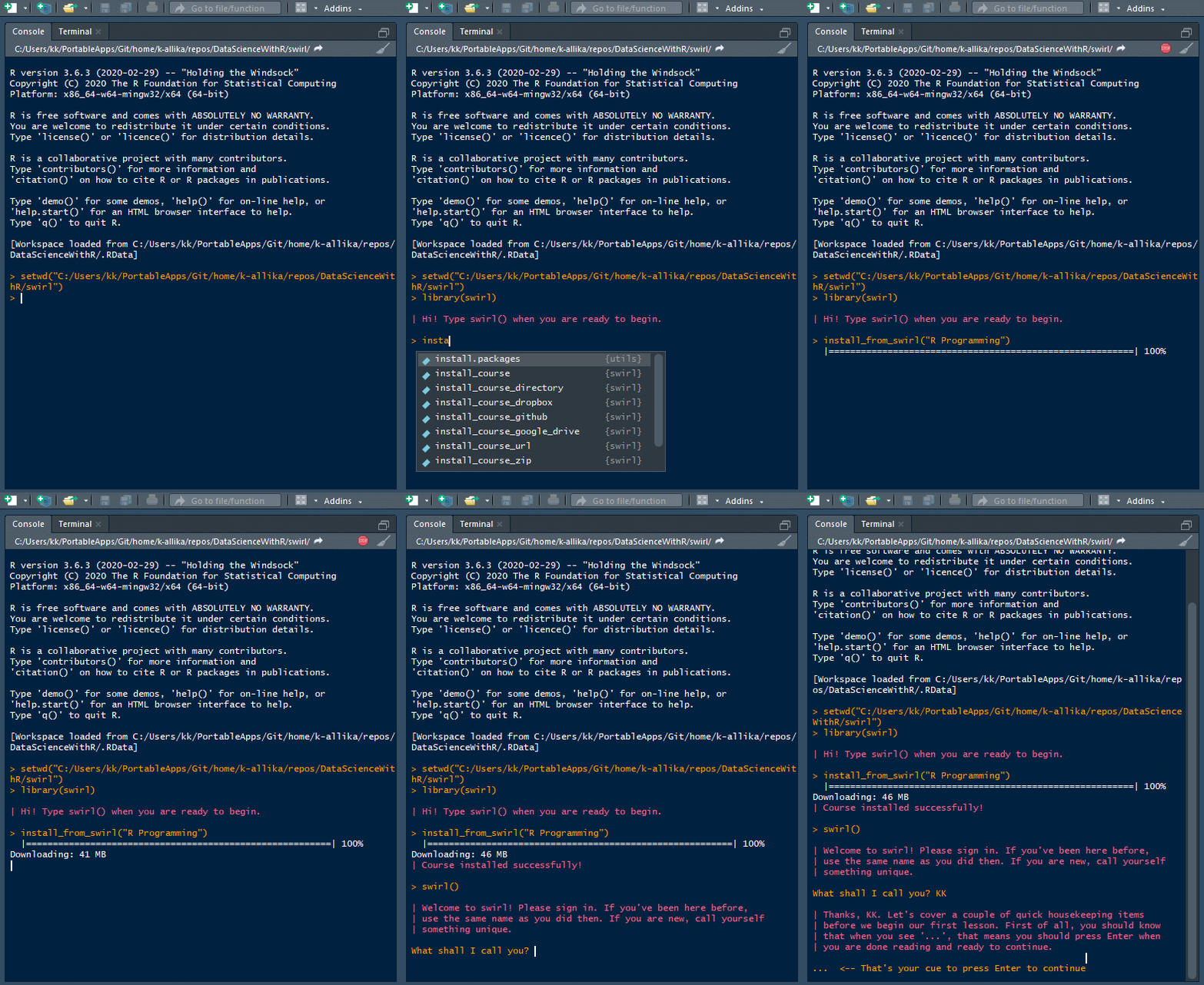
install_from_swirl("R Programming")

Here is a list of all swirl courses http://swirlstats.com/scn/title.html

Installing course

[^top]

Last updated 2020-04-14 09:34:33.536108 IST

GitHub and Git basics

Krishnakanth Allika

2020-04-11 17:03

cache/posts/00300git_basics.html

Contents

GitHub/GitLab Account ¶

GitHub is a service where you can host your projects online with a lot of free features especially for version control. GitHub is also the most popular Git based online repository service followed by GitLab. Click on the hyperlinks to sign up for a free account.

[^top]

Creating a repository ¶

Login to GitHub and select "New Repository". Give a name to your repository(also called repo). Select option "Public" or "Private" depending on whether you want to share your repo with others or not.

[^top]

Installing Git ¶

Download and install Git for Windows from https://git-scm.com/download/win. You can install the regular version or the portable version of from the links on the page. By now, you might have guesed that I have installed the portable version.

[^top]

Connecting R Studio to GitHub ¶

JHU's Linking GitHub and RStudio document shows in detail how to connect R Studio to your GitHub account, create projects in repositories, commit and push repos. Hence, I am not going to go through that here. Also, I am not a big fan of using R Studio to perform Git operations. I believe that one needs to work on CLIs (like Git Bash) to learn and understand how Git versioning works.

[^top]

Git Bash ¶

Git Bash is a CLI(Command Line Interface) for Git operations for Git based online services like GitHub or GitLab. We have already installed Git earlier which contains an executable file called Git Bash. We will use Git Bash to connect to GitHub and perform Git operations.

1. Git Credential Manager for Windows (GCMW)¶

Git Bash can connect to Github via SSH or HTTPS. GitHub recommends HTTPS over SSH as the connections are much faster and easier to set up. To connect over HTTPS, we need to install Git Credential Manager for Windows (GCMW). GCMW provides secure Git credential storage for Windows with Two-factor authentication for GitHub. Download and install the latest GCMW from https://github.com/Microsoft/Git-Credential-Manager-for-Windows/releases/latest

2. Git Bash first time configuration¶

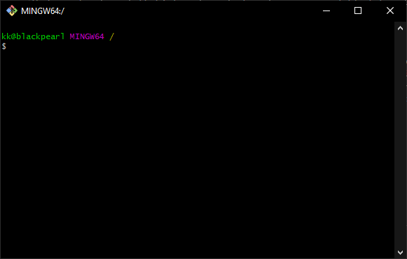
Here are a few things that you need to do when you first install Git. Open Git Bash and you'll see a CLI that looks like this.

Git Bash

1. Type the following command in Git Bash and enter your GitHub username (the one created while setting up the GitHub account) in quotes.

git config --global user.name "YourUserName"

2. Enter your email address associated with your GitHub account.

git config --global user.email [email protected]

3. Configure your favorite text editor for Git Bash. If you installed portable Notepad++ like me, you can configure it as your default Git Bash text editor by typing the following. Edit Notepad++ path accordingly.

git config --global core.editor "'C:/Users/kk/PortableApps/Notepad++Portable/App/Notepad++/notepad++.exe' -multiInst -notabbar -nosession -noPlugin"

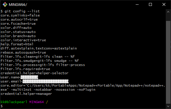
You can also check your settings by entering the following. If something's wrong, use the above commands to change them.

git config --list

Git config

3. Basic Git operations¶

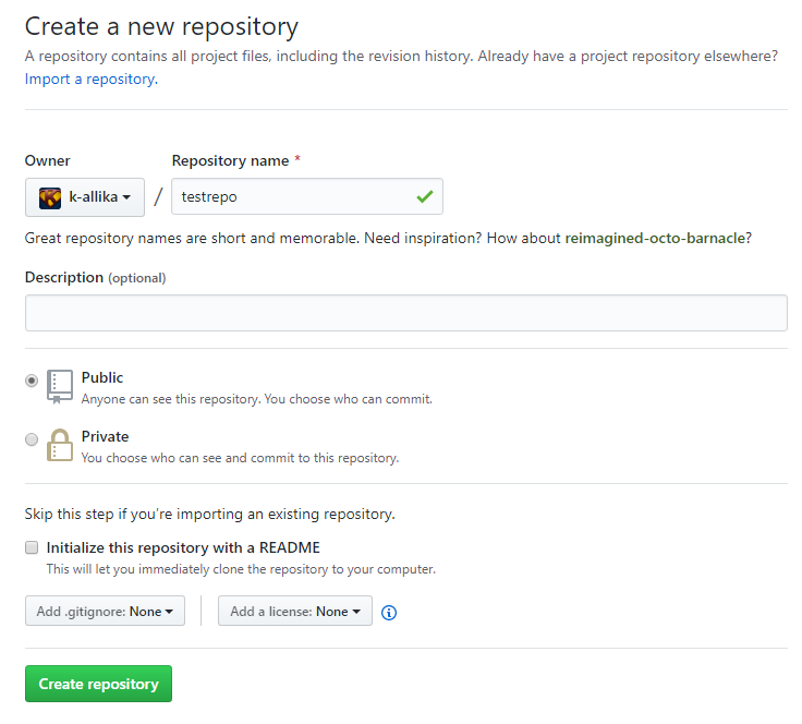
Let's create a repository called "testrepo" and perform some basic Git operations on it. Login to GitHub and create the repository called "testrepo".

Create repo

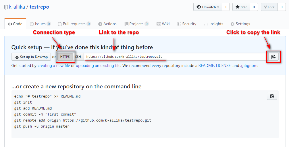
Ensure that the connection is HTTPS. Click copy button to copy the repo link.

Copy repo link

Go to Git Bash and create a directory where you plan to work on your projects. Let's call it "projects".

mkdir projects

Enter the following command to view all files and directories in the current location. One of them should read "projects"

Change directory to "projects"

cd projects

git clone¶

Clone your repo to your current working directory.

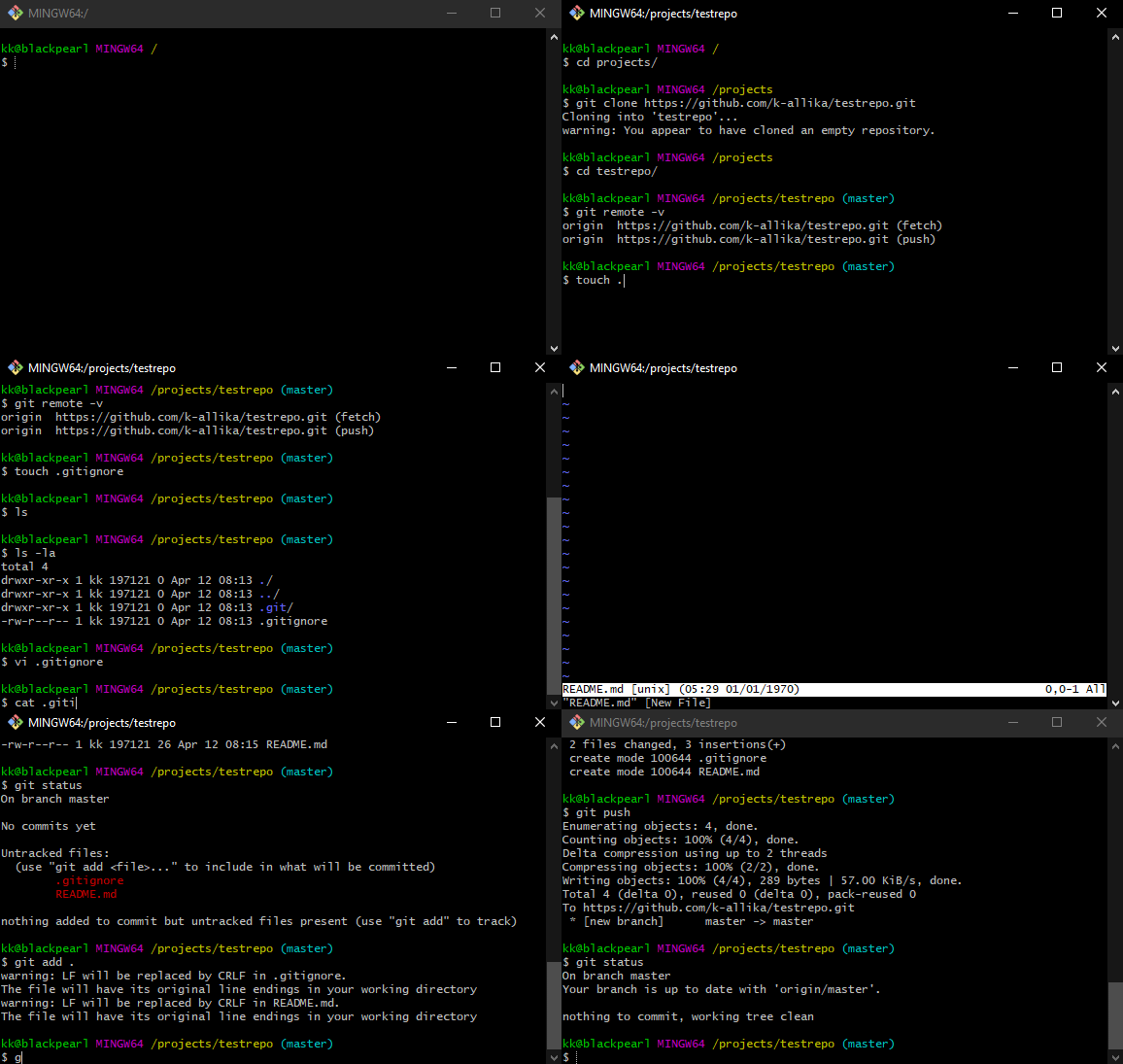
git clone https://github.com/k-allika/testrepo.git

git remote¶

Check connection to your remote repo

git remote -v

.gitignore¶

.gitignore is an important file and should be created before the first push. .gitignore contains a list of files that git will ignore while performing git operations. For example, if I have some text files in my working directory that I do not want to push them to my GitHub repo, then I'll include *.txt in my .gitignore.

touch¶

Create an empty .gitignore file

touch .gitignore

vi¶

Edit an existing file or create a new file and edit.

vi .gitignore

adding *.txt to ignore will tell Git to ignore all txt files and not to push them to remote repo.

Basic vi commands:

i to start editing.

Esc to stop editing and come out of edit mode.

:w to save file.

:q to quit vi

Let's create a "notes.txt" file to test .gitignore. Since we added *.txt to .gitignore, "notes.txt" would not be pushed to the repo.

vi notes.txt

Let's create another file called "README.md". Since this file does not match anything in .gitignore, it would be pushed to the repo.

vi README.md

ls¶

ls lists files and directories in the current directory. The arguments -la will show file attributes along with hidden files.

ls -la

git status¶

View the status of your working directory compared to the remote repo at GitHub.

git status

As expected, you'll notice that only .gitignore and README.md files are mentioned in the status output. The notes.txt is ignore as it should.

git push¶

git push

Push changes in your working directory to the remote repo.

Git Bash Basics

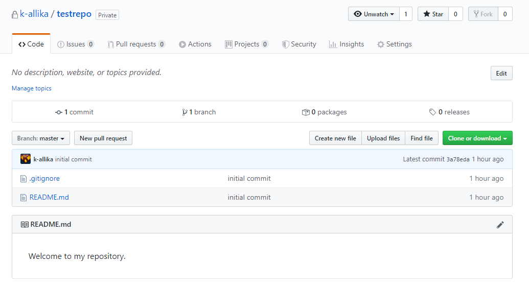
Check your repo at GitHub and you should see the changes there.

Remote repo

[^top]

Last updated 2020-04-13 22:32:36.916238 IST

Installing R and RStudio

Krishnakanth Allika

2020-04-10 10:59

cache/posts/00200install_r.html

Contents

Portable environment ¶

This page will guide you on installing R and RStudio in a portable environment on a Windows 10 system. Following are the reasons why I prefer a portable installation over a regular installation:

I am not tied up to a particular computer. Installation and files reside in a portable drive (a pen-drive or a portable hard disk drive). I can use R on any Windows system wherever I go.
If this system crashes, I don't lose my setup or files.
I like experimenting.

If you prefer a regular installation, visit RStudio and follow the steps.

Installing PortablaApps platform (optional): Portable Apps platforms comes with it's own start menu launcher which is handly when you install multiple portable programs in future. Download and install PortableApps Platform from https://portableapps.com/download.

1. Select "New Install"

2. Select

Portable apps if you want to install it on your pen-drive or a portable hard disk drive
Cloud, if you want to intall it in your Dropbox, Google Drive, PCloud, One Drive, etc
Local - It will be installed in your local drive but only you can access the programs. Other Windows users on your system will not be able to access your portable applications. This is where I am installing.
Local All Users - It will be installed in your local drive and all users on your computer can access them.

Installation options

3. Select your preferred directory and continue. Select directory

Once the installation is complete, open Portable Apps platform and if everthing went well, you'll see something like this. PortableApps

[^top]

Installing R ¶

1. Download R Portable paf.exe file from https://sourceforge.net/projects/rportable/.

2. Open PortableApps Menu and go to Apps > Install a New App

3. Select the R Portable paf.exe file you downloaded earlier and continue installation with default settings.

4. Once installation is complete, you will be able to see R in your Portable Apps menu. Click on it and open R console. Open R

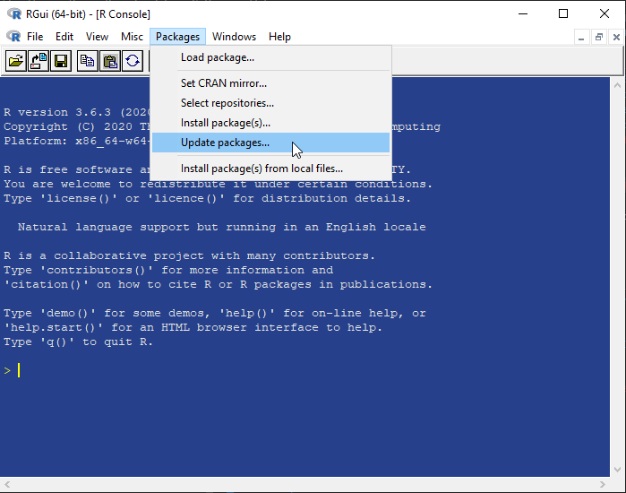
5. Updating R packages: In R Console menu, go to Packages > Update Packages

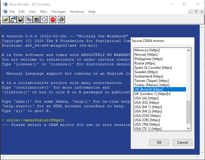
6. Select the CRAN mirror location nearest to you.

7. If there are any packages that need to be updated, you'll see a small window with a list of apps selected. Click 'OK' and update them.

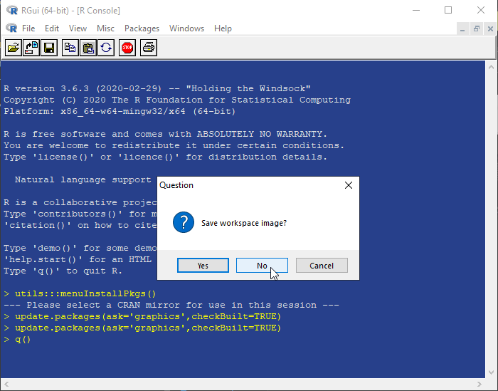
8. Close R console. There is no need to save the workspace image.

[^top]

Installing RStudio ¶

RStudio is provides the GUI(Graphics User Interface) and is also the commonly used IDE(Integrated Development Environment) for R.

1. Go to https://sourceforge.net/projects/rportable/files/R-Studio/ and select the latest version of RStudio. Download the paf.exe file from the folder.

2. Open PortableApps Menu and go to Apps > Install a New App

3. Select the RStudio Portable paf.exe file you downloaded earlier and continue installation with default settings.

4. Once installation is complete, you will be able to see RStudioPortable in your Portable Apps menu. Click on it and open R Studio.

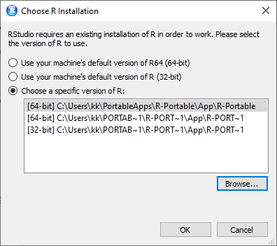
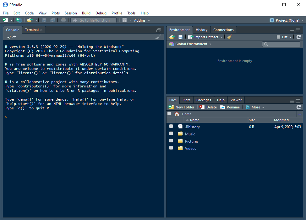
5. The first time you open R Studio, it will ask you to chose the version of R you want to use. select R version

6. Click "Browse" and point to the "bin" directory of portable R you installed earlier. The path looks similar to C:\Users\YourUserName\PortableApps\R-Portable\App\R-Portable\bin.

7. Select 32-bit or 64-bit based on your Windows 10 version. If you are unsure, select 32-bit as it works on both.

You are now ready to use R Studio. RStudio

8.\ Create R Project. Select File > New Project. Select "New Directory".

New Directory

Select "New Project"

New Project

Name your project (example: DataScienceWithR). Browse and select the directory where you want the project to reside. Click "Create Project".

Project name and location

You should now see your project files including "DataScienceWithR.Rproj" file in the second quadrant of R Studio.

[^top]

Installing R Markdown ¶

As a data scientist, it's important to not only write and run code but also explain data manipulation and inferences in words. Markdown allows us to document our work. R-Markdown integrates R code with Markdown to provide an integrated solution. JupyterLab (a successor of iPython) is another such tool, which we will come across soon.

1.\ In R Studio, go to File > New File > R Markdown.

2.\ If there are any missing packages, R Studio will ask you if you'd like to install them. Click 'OK' and wait for it to install.

Installing R Markdown dependencies

3.\ Give a name to the document (example: sample). Select 'HTML' or 'PDF' as your choice of output.

R Markdown options

4.\ This will create a sample markdown document with some examples in it. You may change the 'title' in the document to "Sample Markdown". Save the file.

Sample Markdown

5. Press CTRL+SHIFT+K or click the "Knit" button in the fourth quadrant of R Studio or go to File > Knit Document to generate an HTML or PDF output of the markdown file.

HTML output

[^top]

Installing R in JupyterLab (Optional)¶

This step is completely optional and you can safely skip it. JupyterLab is a web-based interactive development environment for Jupyter notebooks, code, and data. It supports over 40 programming languages including R. I started using JupyterLab a short time ago while learning Python and am quite impressed by its features, interactivity, improvements and its community. This is my attempt to run R in JupyterLab environment.

Follow the steps to install R in JupyterLab. If you already have JupyterLab installed, you can directly go to step x.

1. Anaconda vs Miniconda: To use JupyterLab, you need to have Anaconda or Miniconda installed. Follow either 1a or 1b.

1a. Anaconda comes bundled with Python and a lot of packages commonly used in data science. It also comes with a GUI called Navigator and it's own IDE called Spyder. If you are a beginner, install Anaconda from https://www.anaconda.com/distribution/. Select Python 3+ version. Install will default settings.

1b. Miniconda is a small, bootstrap version of Anaconda that includes only conda, Python, the packages they depend on, and a small number of other useful packages. I prefer Miniconda instead of Anaconda as I don't need Anaconda's GUI and IDE and I am more comfortable with using CLI(Command Line Interface) for installing and maintaining packages. Also, I don't need all the packages that come with Anaconda. I can install the packages I want when I need them. Download Miniconda from https://docs.conda.io/en/latest/miniconda.html. You can install with default settings, or if you prefer a portable version of it, open the command prompt in administrator mode and go to the directory where you downloaded Minoconda exe file and type the following

Miniconda3-latest-Windows-x86_64.exe /InstallationType=JustMe /AddToPath=0 /RegisterPython=0 /NoRegistry=1

2. Creating a virtual environment: In Anaconda(or Miniconda. In future, I am going to use the term Anaconda for both Anaconda and Miniconda because they both have the same core. Whatever works in one, works in the other too.), we have an option to create virtual environments. Each environment can have packages and code specific to its project. This is useful because different projects require different packages and it's not advisable to install all packages at one place in the base(base is the default environment that comes with Anaconda). Also, if you don't want to mess up the base when you are experimenting. Always create a new environment, experiment and if something goes wrong then delete it and create a new one without having to reinstall Anaconda.

2a. Open 'Anaconda Prompt' from Windows Start Menu

2b. Create a virtual environment. Enter the following in the command prompt.

conda create --name jhu.

I created an environment called 'jhu'. The name is arbitrary. You can name it anything you want.

Create a virtual environment

2c. Activate the virtual environment

conda activate jhu

Replace 'jhu' with your environment name. You should see the name of the environment in brackets on the left of the prompt.

Activate the virtual environment

3. Install JupyterLab

conda install -c conda-forge jupyterlab

This will show a list of dependency packages to be installed. Press 'y' and continue.

4. Install R in JupyterLab

conda install -c r r-essentials

This will install R along with essential packages to use R in JupyterLab. Now open JupyterLab by typing the following

jupyter lab

If everywthing went well, you should see JupyterLab launcher with R installed alongside Python.

R kernel in JupyterLab

Let's run a small piece of R code that I copied from here and see if it works.

In [2]:

library(dplyr)
library(ggplot2)
ggplot(data=iris, aes(x=Sepal.Length, y=Sepal.Width, color=Species)) + geom_point(size=3)

Works well!

[^top]

Last updated 2020-04-11 16:47:25.910599 IST

Introduction to data science

Krishnakanth Allika

2020-04-09 12:34

cache/posts/00100intro_ds.html

Contents

Data science ¶

Data science involves statistics, computer science and mathematics.
Machine learning and artificial intelligence are two of the most popular branches of data science these days.
Three key features of Big Data
- Volume - Deals with huge amounts of data.
- Velocity - Data is generated rapidly, also involves real time data.
- Variety - Deals with structured and unstructured data.

Three Vs of Big Data

A data scientist is someone who applies data science tools to data to answer questions.
Data scientists usually have a combination of the following skills:

Data scientist's skills

[^top]

Data ¶

There are several definitions of data. The definition provided by Wikipedia is "A set of values of qualitative or quantitative variables".

Definition of data

There are two kinds of data we usually come across:

Structured data - Data that can be stored in tabular format (rows and columns) and each variable (or column) has a specific data type (numeric, text, category, etc)
Unstructred data - Any data that is not structured is unstructed data. Some examples are twitter data, facebook comments, sequencing data (medical, genome data), medical records, languages, images, etc

Variables

Quantitative - measureable, numeric (integers or real numbers).
- examples: age, distance, time, etc
Qualitative - non-measurable (example: categorical or user assigned)
- examples: name, severity(High, Medium, Low), ranking, etc
Quantitative variables can be discrete or continuous*.

[^top]

Data science project ¶

Steps or life cycle of a data science project

Business case (forming a question, scope analysis)
Data collection (finding or generating data)
Data pruning (data cleansing, data manipulation, data visualization)
Data analysis (Exploratory and/or Inferential statistics)
Data Modeling (Machine Learning, Artificial Intelligence)
Closure (Conclusions, reporting, communication to stakeholders, future scope)

[^top]

* Johns Hopkins University course stated that "Quantitative variables are measured on ordered, continuous scales", which, in my opinion, is a vague statement. Quantitative variables are measured not only on continuous scales but also on discrete (non-continous) scales. Some examples of discrete quantitative variables are 'age in years', 'number of days since first medication', 'number of pencils in a box', etc

Last updated 2020-04-13 22:35:12.176242 IST