COVID-19 data
JHU exercise data 
Disclaimer: This exercise is to help people understand data sclicing operations in R. I will not be providing solutions to JHU assignments. However, these exercises will help get closer to finding solutions.
Data is provided in the form of a URL containing a zip file. There are more than one ways to extract data from zip files.
Data extraction - Method 1
- Download zip file into working directory.
- Decompress the zip file into working directory.
- Check data file format.
- Load decompressed file into a dataframe.
Disadvantage: Will end up with two files (a zip file and a data file) in the working directory which are unnecessary.
# Download the dataset from the URL to the working directory and name it as "data.zip"
download.file("https://d396qusza40orc.cloudfront.net/rprog/data/quiz1_data.zip","data.zip")
#unzip the zip file to a directory called "data"
unzip("data.zip",exdir="data")
# List file in the "data" directory to check data file format
list.files("data")
The data is available in a CSV (comma seperated values) file. We will use read.csv to read data into a dataframe.
# Reading data into a dataframe called "df"
df_data1<-read.csv("data/hw1_data.csv")
# View sample data.
head(df_data1)
Data extraction - Method 2
Earlier, we ended up with two unnecessary files and a directory in our working directory. Let's try another way to extracting data without downloading anything to our working directory.
- Download zip file into kernel/memory.
- Check data file format.
- Load data file into a dataframe.
# Create an empty file in memory
file<-tempfile()
# Download the zip file to this empty file
download.file("https://d396qusza40orc.cloudfront.net/rprog/data/quiz1_data.zip",file)
# Check data file format
unzip(file,list=TRUE)
# Load data file to dataframe
df_data<-read.csv(unz(file,"hw1_data.csv"))
# Delete file from memory
unlink(file)
# View sample data
head(df_data)
Checking if both dataframes are identical
identical(df_data,df_data1)
# Dimensions of the dataframe
dim(df_data)
df_data has 153 rows and 6 columns.
Let's write the same in data science langauge:
The dataframe contains 153 records of 6 variables or features.
# View the first 3 records of te dataframe to get an idea about the data in it.
head(df_data, n=3)
# View the last four records.
tail(df_data,n=4)
We can also find the number of records by finding the length of any one of the variables (example, Ozone)
length(df_data$Ozone)
Data slicing (also called subsetting in R) is done using the [ function. The standard syntax is [rows,columns]. If we need to slice by rows, we can omit columns like [rows,]. Do not forget the trailing comma because without it, R assumes that we are slicing by columns by default or slicing a vector.
# Ozone level of 29th row
df_data[29,"Ozone"]
If the variables of a dataframe are named, then we can also use their names the following way to achieve the same result as above.
# Ozone level of 29th row
df_data$Ozone[29]
How did this work? When we call a variable of a dataframe, it becomes a vector. Here df_data$Ozone is an integer vector. We viewed the 29th element of the vector.
class(df_data$Ozone)
Missing values: is.na() provides a logical vector of missing values - TRUE if NA and FALSE if not NA. In R, TRUE = 1 and FALSE = 0. A sum function will output the sum of all TRUE values (or missing values).
Number of missing values in variable Solar.R:
# Number of missing values in variable Solar.R
sum(is.na(df_data$Solar.R))
Mean of the variable Solar.R excluding missing values:
# Mean of the variable Solar.R excluding missing values
mean(df_data$Solar.R, na.rm=TRUE)
Mean of Solar.R where Ozone levels are lower than 25 and Temp is below 88:
# Mean of Solar.R where Ozone levels are lower than 25 and Temp is below 88.
mean(df_data$Solar.R[df_data$Ozone<25&df_data$Temp<88],na.rm=TRUE)
Average Ozone level in the month of May:
# Average Ozone level in the month of May
mean(df_data$Ozone[df_data$Month==5], na.rm=TRUE)
Maximum Solar Radiation in June:
# Maximum Solar Radiation in June
# More info on usage of max() function: http://www.endmemo.com/program/R/max.php
max(df_data$Solar.R[df_data$Month==6],na.rm=TRUE)
[^top]
COVID data by JHU CSSE 
Source: https://github.com/CSSEGISandData/COVID-19
Data URL: http://link.datascience.eu.org/p003d1
Data last updated: 2020-04-13
# Loading data to dataframe
df_JHU<-read.csv("http://link.datascience.eu.org/p003d1")
head(df_JHU, n=2)
Pruning dataframe by stripping away unrequired variables:
We only need Country, State, Confirmed, Deaths, Recovered and Active.
df_JHU<-df_JHU[,c("Country_Region","Province_State","Confirmed","Deaths","Recovered","Active")]
head(df_JHU,n=2)
Confirmed cases, deaths and death rates in US and India vs Global:
# Confirmed cases
c_US<-sum(df_JHU[df_JHU$Country_Region=="US","Confirmed"])
c_IN<-sum(df_JHU[df_JHU$Country_Region=="India","Confirmed"])
c_GL<-sum(df_JHU["Confirmed"])
c<-c(c_US,c_IN,c_GL)
# Deaths
d_US<-sum(df_JHU[df_JHU$Country_Region=="US","Deaths"])
d_IN<-sum(df_JHU[df_JHU$Country_Region=="India","Deaths"])
d_GL<-sum(df_JHU["Deaths"])
d<-c(d_US,d_IN,d_GL)
# Death rates
dr<-d/c*100
# Creating a dataframe
df_dr<-cbind(Country=c("US","India","Global"),Confirmed=c,Deaths=d,Death_Rate=dr)
df_dr
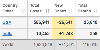
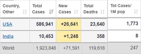
The numbers are close to the reports from https://www.worldometers.info/coronavirus/
[^top]
COVID data by Kaggle 
Source: https://www.kaggle.com/sudalairajkumar/novel-corona-virus-2019-dataset/data
Data URL: http://link.datascience.eu.org/p003d2
Data last updated: 2020-04-13
df_kaggle<-read.csv("http://link.datascience.eu.org/p003d2")
head(df_kaggle,n=2)
Pruning dataframe by stripping away unrequired variables:
We only need Country, State, Confirmed, Deaths, Recovered.
df_kaggle<-df_kaggle[,c("Country.Region","Province.State","Confirmed","Deaths","Recovered")]
head(df_kaggle,n=2)
Confirmed cases, deaths and death rates in US and India vs Global:
# Confirmed cases
c_US<-sum(df_kaggle[df_kaggle$Country.Region=="US","Confirmed"])
c_IN<-sum(df_kaggle[df_kaggle$Country.Region=="India","Confirmed"])
c_GL<-sum(df_kaggle["Confirmed"])
c<-c(c_US,c_IN,c_GL)
# Deaths
d_US<-sum(df_kaggle[df_kaggle$Country.Region=="US","Deaths"])
d_IN<-sum(df_kaggle[df_kaggle$Country.Region=="India","Deaths"])
d_GL<-sum(df_kaggle["Deaths"])
d<-c(d_US,d_IN,d_GL)
# Death rates
dr<-d/c*100
# Creating a dataframe
df_dr<-cbind(Country=c("US","India","Global"),Confirmed=c,Deaths=d,Death_Rate=dr)
df_dr
The numbers are way off compared to the reports from https://www.worldometers.info/coronavirus/. The source data needs to be checked.
[^top]
COVID by EU Open Data Portal 
Source: https://opendata.ecdc.europa.eu/covid19/casedistribution/csv
Data URL: http://link.datascience.eu.org/p003d3
Data last updated: 2020-04-14
df_EU<-read.csv("http://link.datascience.eu.org/p003d3")
head(df_EU,n=2)
Pruning dataframe by stripping away unrequired variables:
We only need Country, cases, deaths, population.
df_EU<-df_EU[,c("countriesAndTerritories","cases","deaths","popData2018")]
head(df_EU,n=2)
Confirmed cases, deaths, death rates and cases per million population in US and India vs Global:
# cases cases
c_US<-sum(df_EU[df_EU$countriesAndTerritories=="United_States_of_America","cases"])
c_IN<-sum(df_EU[df_EU$countriesAndTerritories=="India","cases"])
c_GL<-sum(df_EU["cases"])
c<-c(c_US,c_IN,c_GL)
# deaths
d_US<-sum(df_EU[df_EU$countriesAndTerritories=="United_States_of_America","deaths"])
d_IN<-sum(df_EU[df_EU$countriesAndTerritories=="India","deaths"])
d_GL<-sum(df_EU["deaths"])
d<-c(d_US,d_IN,d_GL)
# Death rates
dr<-d/c*100
# Population
p_US<-df_EU[df_EU$countriesAndTerritories=="United_States_of_America","popData2018"][1]
p_IN<-df_EU[df_EU$countriesAndTerritories=="India","popData2018"][1]
p_GL<-7631091112     # World pop in 2018 per https://www.populationpyramid.net/world/2018/
p<-c(p_US,p_IN,p_GL)
# Cases per million population
cpm<-c/p*1000000
# Creating a dataframe
df_dr<-cbind(Country=c("United_States_of_America","India","Global"),cases=c,deaths=d,Death_Rate=dr, Cases_per_Mil=cpm)
df_dr
The numbers are close to the reports from https://www.worldometers.info/coronavirus/
[^top]
Last updated 2020-04-15 11:52:46.054857 IST
Comments